Many models, same data

Introduction

Let’s talk about model selection! As a non-statistician, I find the process of choosing an appropriate statistical model to be slightly intimidating, even agonizing at times. In the hopes of demystifying this process for other non-statisticians, this post attempts to walk you through how Gina Nichols and I decided on the appropriate models and stats for an upcoming manuscript. Constructive feedback is always welcome.

Gina and I are using data from this project. In very brief terms we’re interested in the effect of cover crops on the weed seed bank of corn/soybean cropping systems. While cover crops are oft cited as a practice than can help decrease erosion or nutrient export from agricultural fields, we are curious if using cover crops can help decrease the weed seed bank. This is especially important because of the increasing prevalence of herbicide resistant weeds across the Midwest (and beyond).

Data

The data can be accessed from Gina Nichols’ Github repository like so:

remotes::install_github("vanichols/PFIweeds2020")

The raw data are in the data-frame pfi_ghobsraw. These are observations from soil collected at each site which Gina then incubated in a greenhouse to grow weeds. We don’t need to clean the data very much, but we will do a couple steps to consolidate observations.

A couple other notes on the experimental layout:

• There are four site_sys, which encompass three different farms and two different cropping systems
  • Boyd Grain
  • Boyd Silage
  • Funcke Grain
  • Stout Grain

FYI: Grain systems employ a two year rotation of corn and soybeans and sell both crops off as feed grain, ethanol grain, etc. The silage system also has a 2 year rotation of corn and soybeans, but in the corn year the crop is harvested earlier (while it’s still green) and sold as silage (fermented cattle feed)

• There are two cover crop treatments cc_trt = none and cc_rye= rye
• There are 4-5 blocks per treatment, which will be our random effect.

Library loading & initial data visualization

library(dplyr)
library(lme4)
library(lmerTest)
library(ggResidpanel)
library(performance)
library(ggplot2)
library(patchwork)
library(PFIweeds2020)
theme_set(theme_bw())

A couple notes about the libraries we used:

• We are fitting models using lme4 and lmerTest packages.
• We are using two different packages to examine model fit/diagnostics.
  • ggResidpanel has much improved versions of model diagnostic plots. Would highly recommend!
  • performance also has improved model diagnostic plots as well as simple ways of calculating R² for fixed & random effects and checking for over-dispersion.

data("pfi_ghobsraw")

# Quick data cleaning
dat <- 
  pfi_ghobsraw %>% 
  dplyr::mutate_if(is.numeric, tidyr::replace_na, 0) %>%
  dplyr::group_by(site_name, field, sys_trt, cc_trt, rep, blockID) %>%
  dplyr::summarise_if(is.numeric, sum) %>%
  dplyr::ungroup() %>%
# Sum all seeds by species  
  dplyr::mutate(totseeds = rowSums(.[, 7:24])) %>%
  tidyr::unite(site_name, sys_trt, col = "site_sys", remove = T) %>% 
  select(-field, -rep, -c(AMATU:UB)) %>%
  mutate(cc_trt = recode(cc_trt,         
                          no = "none",
                          rye = "cc_rye"))
head(dat)

## # A tibble: 6 x 4
##   site_sys   cc_trt blockID totseeds
##   <chr>      <chr>  <chr>      <dbl>
## 1 Boyd_grain none   B42_1         34
## 2 Boyd_grain none   B42_2         12
## 3 Boyd_grain none   B42_3          9
## 4 Boyd_grain none   B42_4          7
## 5 Boyd_grain none   B42_5         17
## 6 Boyd_grain cc_rye B42_1        116

We are interested in totseeds (total seeds) as a response variable, which is an integer value. In all of our mixed models our fixed effects are site_sys and cc_trt and our random effect is blockID.

But before we get to modeling, let’s just quickly look at the data and see what we are working with.

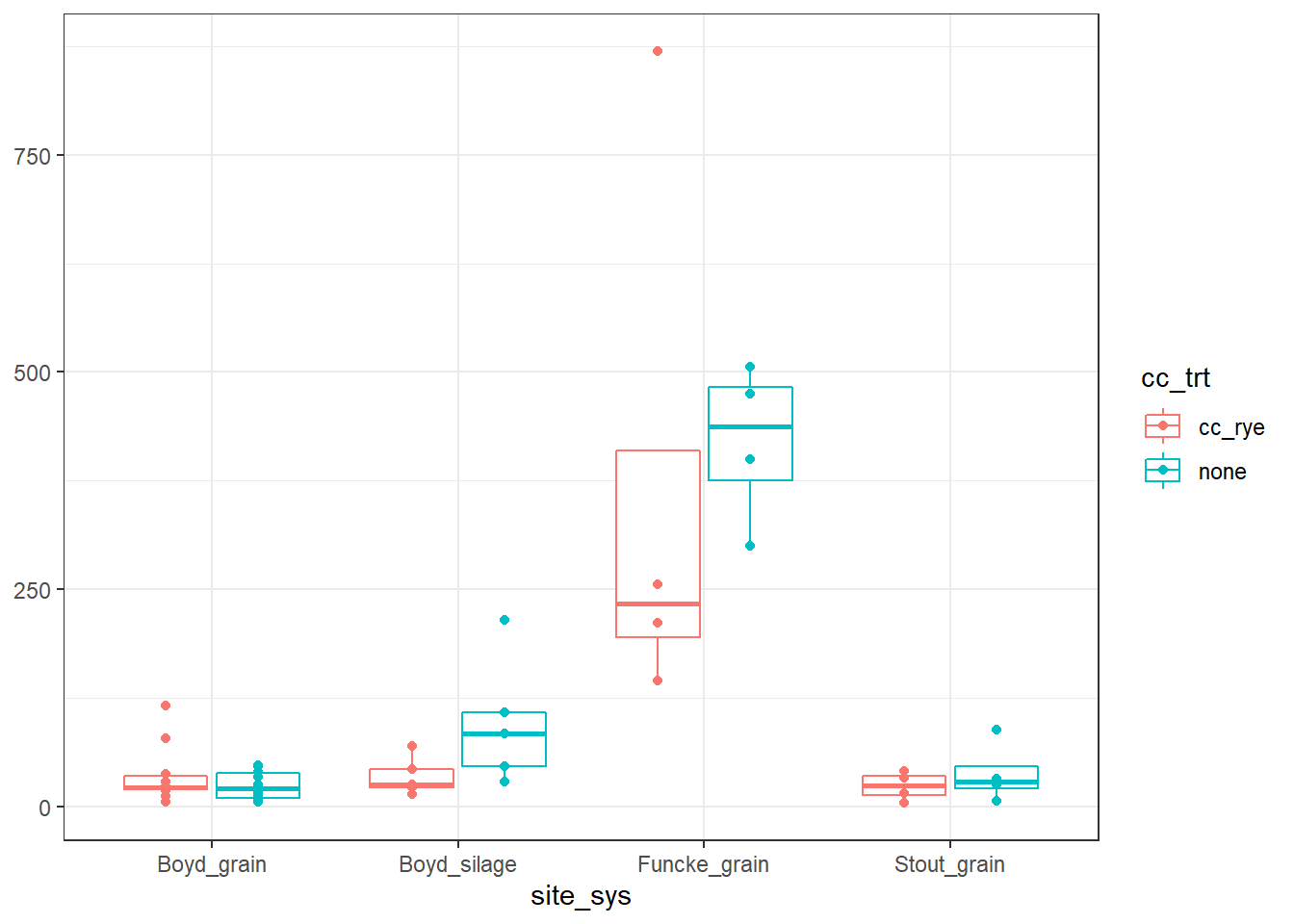There is one point that is much higher than the rest, in the Funcke_grain cover crop treatment, which may be a little cause for concern…we’re going to make another data-set without it.

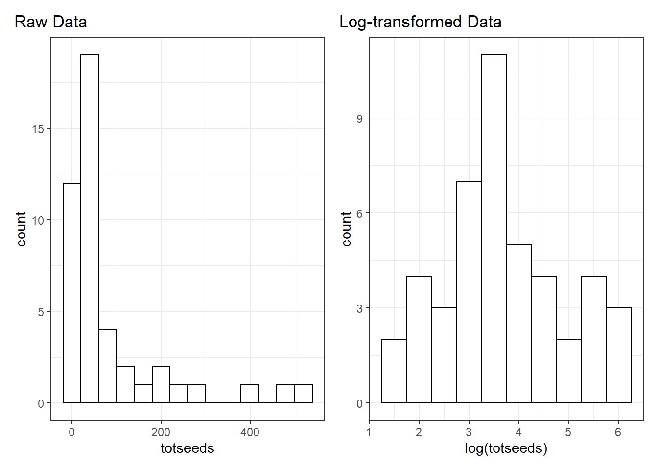
dat2 <- dat %>%
  filter(totseeds < 700)

Let’s also plot the distribution of totseeds. It is pretty skewed. If we log-transform the raw data we get a much nicer distribution and our large values are much less far apart than our small values.

Model fitting

OK now it’s time to start fitting out models. Given the graphs above, our first thought was to run a lmer with a log-transformed response.

(Here we are also examining whether there is any interaction between site_sys and cc_trt, and looks like there is. We are therefore going to keep the interaction in all the models going forward)

m1 <- lmer(log(totseeds) ~ site_sys * cc_trt + (1|blockID), data = dat2)
m2 <- lmer(log(totseeds) ~ site_sys + cc_trt + (1|blockID), data = dat2)

anova(m1, m2) # keep interaction

## Data: dat2
## Models:
## m2: log(totseeds) ~ site_sys + cc_trt + (1 | blockID)
## m1: log(totseeds) ~ site_sys * cc_trt + (1 | blockID)
##    npar    AIC    BIC  logLik deviance  Chisq Df Pr(>Chisq)  
## m2    7 117.40 130.04 -51.698  103.397                       
## m1   10 115.13 133.20 -47.566   95.132 8.2643  3    0.04085 *
## ---
## Signif. codes:  0 '***' 0.001 '**' 0.01 '*' 0.05 '.' 0.1 ' ' 1

Before we dive into the summary values and statistical reporting lets check out our diagnostic plots:

ggResidpanel::resid_panel(m1)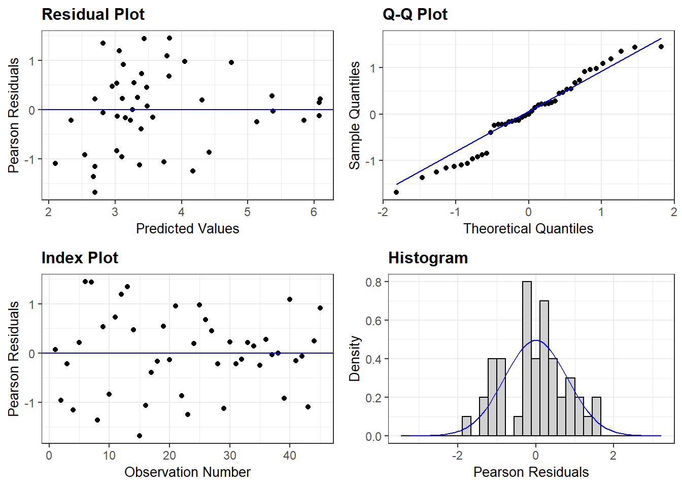

This doesn’t look bad, but perhaps it could look better…

To stick within the normal-distribution framework we could also try another transformation. The square-root transformation can also work for count data.

dat %>%
  ggplot(aes(sqrt(totseeds)))+
  geom_histogram(binwidth = 1, fill = "white", color = "black")+
  ggtitle("Sqrt-transformed Data")+
  theme(plot.title.position = "plot")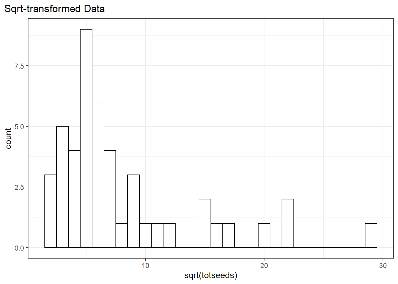

The data still look a little skewed, but that’s OK…

m1b <- lmer(sqrt(totseeds) ~ site_sys * cc_trt + (1|blockID), dat2)
resid_panel(m1b)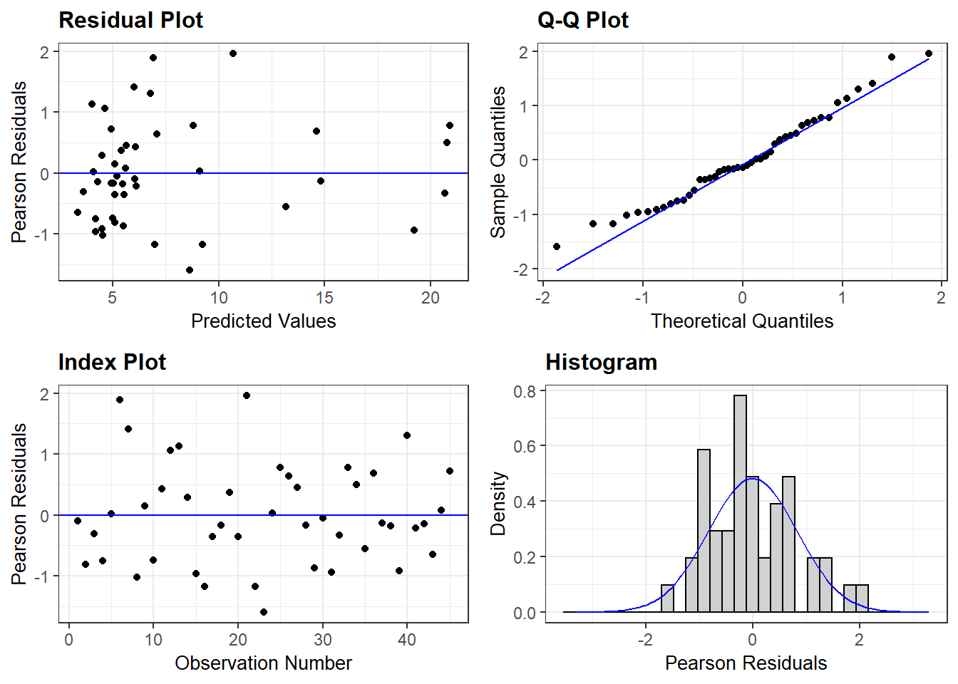

These diagnostic plots look pretty similar, although the square root transformation might be a little better. The problem with the square root transformation is that it renders the data pretty uninterpretable and we’d like to be able to interpret our model estimates.

Since we are working with count data, however, we have other options in our stats toolbox - generalized linear models. We don’t even need to load another package to do this, we just need to call glmer from the {lme4} package and specify which distribution we’re fitting.

Our first attempt with glmer will be a Poisson distribution, which is meant for count data and often (but not always) uses a log link function.

p1a <- glmer(totseeds ~ site_sys*cc_trt + (1|blockID), data = dat2, 
            family = poisson(link = "log"))

It looks like our model successfully fit the data. But we should always check for over-dispersion in our Poisson models, which is when the variance >> mean.

performance::check_overdispersion(p1a) 

## # Overdispersion test
## 
##        dispersion ratio =   8.001
##   Pearson's Chi-Squared = 288.047
##                 p-value = < 0.001

## Overdispersion detected.

Just as an aside, you can also calculate dispersion by hand using one of these two methods:

# option 1
1 - pchisq(deviance(p1a), df.residual(p1a)) 

## [1] 0

# option 2
r <- resid(p1a,type="pearson")
1-pchisq(sum(r^2),df.residual(p1a))

## [1] 0

Either way our p-value is very close to 0, so it looks like our data are over-dispersed.

Now we have two options if we want to continue down the glmer path. We could:

1. Add an observation-level random effect to our Poisson model.

2. Switch to a different distribution, like the negative binomial.

Let’s start with option 1 and add an observation-level random effect. To learn more about why this helps, see this article.

dat2 <- 
  dat2 %>%
  mutate(obs_id = paste("obs", 1:n(), sep = "_"))

p1b <- glmer(totseeds ~ site_sys*cc_trt + (1|blockID) + (1|obs_id), data = dat2, 
            family = poisson(link = "log"))

performance::check_overdispersion(p1b)

## # Overdispersion test
## 
##        dispersion ratio = 0.145
##   Pearson's Chi-Squared = 5.065
##                 p-value =     1

## No overdispersion detected.

Adding our observation-level random effect fixed out over-dispersion problem. Great!

But let’s also try option 2 and fit the data to a negative-binomial model.

# option 2, negative binomial....
g1a <- glmer.nb(totseeds ~ site_sys*cc_trt + (1|blockID), data = dat2)

This model also converges, which is great! In my limited experience using negative binomial models this isn’t always true so this is a small victory.

Let’s now compare the summary values of the two models:

summary(p1b)

## Generalized linear mixed model fit by maximum likelihood (Laplace
##   Approximation) [glmerMod]
##  Family: poisson  ( log )
## Formula: totseeds ~ site_sys * cc_trt + (1 | blockID) + (1 | obs_id)
##    Data: dat2
## 
##      AIC      BIC   logLik deviance df.resid 
##    445.2    463.2   -212.6    425.2       35 
## 
## Scaled residuals: 
##      Min       1Q   Median       3Q      Max 
## -0.95403 -0.21021 -0.00504  0.16007  0.43396 
## 
## Random effects:
##  Groups  Name        Variance Std.Dev.
##  obs_id  (Intercept) 0.2892   0.5378  
##  blockID (Intercept) 0.1755   0.4189  
## Number of obs: 45, groups:  obs_id, 45; blockID, 18
## 
## Fixed effects:
##                                 Estimate Std. Error z value Pr(>|z|)    
## (Intercept)                      3.28902    0.22578  14.567  < 2e-16 ***
## site_sysBoyd_silage              0.06262    0.32769   0.191  0.84846    
## site_sysFuncke_grain             2.01960    0.44965   4.492 7.07e-06 ***
## site_sysStout_grain             -0.38915    0.42852  -0.908  0.36381    
## cc_trtnone                      -0.31789    0.26083  -1.219  0.22293    
## site_sysBoyd_silage:cc_trtnone   1.26342    0.44048   2.868  0.00413 ** 
## site_sysFuncke_grain:cc_trtnone  1.02944    0.49836   2.066  0.03886 *  
## site_sysStout_grain:cc_trtnone   0.74297    0.48961   1.517  0.12915    
## ---
## Signif. codes:  0 '***' 0.001 '**' 0.01 '*' 0.05 '.' 0.1 ' ' 1
## 
## Correlation of Fixed Effects:
##             (Intr) st_sB_ st_sF_ st_sS_ cc_trt s_B_:_ s_F_:_
## st_sysByd_s -0.450                                          
## st_sysFnck_ -0.502  0.225                                   
## st_sysStt_g -0.525  0.239  0.263                            
## cc_trtnone  -0.565  0.392  0.284  0.298                     
## st_sysBy_:_  0.335 -0.683 -0.168 -0.176 -0.592              
## st_sysFn_:_  0.296 -0.204 -0.628 -0.155 -0.524  0.310       
## st_sysSt_:_  0.301 -0.210 -0.151 -0.580 -0.533  0.316  0.279

summary(g1a)

## Generalized linear mixed model fit by maximum likelihood (Laplace
##   Approximation) [glmerMod]
##  Family: Negative Binomial(3.7588)  ( log )
## Formula: totseeds ~ site_sys * cc_trt + (1 | blockID)
##    Data: dat2
## 
##      AIC      BIC   logLik deviance df.resid 
##    445.4    463.5   -212.7    425.4       35 
## 
## Scaled residuals: 
##     Min      1Q  Median      3Q     Max 
## -1.2879 -0.6244 -0.1260  0.4711  2.0199 
## 
## Random effects:
##  Groups  Name        Variance Std.Dev.
##  blockID (Intercept) 0.179    0.4231  
## Number of obs: 45, groups:  blockID, 18
## 
## Fixed effects:
##                                 Estimate Std. Error z value Pr(>|z|)    
## (Intercept)                      3.43950    0.22667  15.174  < 2e-16 ***
## site_sysBoyd_silage             -0.01624    0.32432  -0.050  0.96005    
## site_sysFuncke_grain             1.88043    0.44272   4.247 2.16e-05 ***
## site_sysStout_grain             -0.45557    0.42093  -1.082  0.27912    
## cc_trtnone                      -0.32847    0.25796  -1.273  0.20290    
## site_sysBoyd_silage:cc_trtnone   1.35345    0.43192   3.134  0.00173 ** 
## site_sysFuncke_grain:cc_trtnone  1.03593    0.48511   2.135  0.03273 *  
## site_sysStout_grain:cc_trtnone   0.77414    0.47305   1.636  0.10174    
## ---
## Signif. codes:  0 '***' 0.001 '**' 0.01 '*' 0.05 '.' 0.1 ' ' 1
## 
## Correlation of Fixed Effects:
##             (Intr) st_sB_ st_sF_ st_sS_ cc_trt s_B_:_ s_F_:_
## st_sysByd_s -0.464                                          
## st_sysFnck_ -0.513  0.237                                   
## st_sysStt_g -0.518  0.249  0.265                            
## cc_trtnone  -0.574  0.445  0.295  0.298                     
## st_sysBy_:_  0.344 -0.694 -0.176 -0.180 -0.609              
## st_sysFn_:_  0.307 -0.237 -0.625 -0.158 -0.533  0.324       
## st_sysSt_:_  0.316 -0.243 -0.162 -0.564 -0.547  0.333  0.292

performance::compare_performance(p1b, g1a)

## # Comparison of Model Performance Indices
## 
## Model |     Type |    AIC |    BIC | R2_conditional | R2_marginal |  ICC | RMSE | SCORE_LOG | SCORE_SPHERICAL |   BF
## --------------------------------------------------------------------------------------------------------------------
## p1b   | glmerMod | 445.17 | 463.24 |           0.78 |        0.66 | 0.36 | 0.35 |     -2.82 |            0.14 |     
## g1a   | glmerMod | 445.44 | 463.50 |           0.81 |        0.67 | 0.42 | 0.90 |     -4.49 |            0.12 | 0.88

Both these models have very similar AICs, and they also have very similar estimates and p-values which is reassuring, since our interpretation of the data won’t change depending on the model we choose.

In the end we decided to go with the Poisson-observation-level-random-effect model (named here p1b). Poisson models are slightly more simple than negative binomial and built for count data.