Overall notes about the R package gt: I like it! I’m still learning the syntax but it seems intuitive and user-friendly. Would recommend.
It’s worth noting at the beginning of this post that the tables are rendered a little differently via blogdown than they would be if they were just knit into an html file. Therefore, please don’t view this page in dark mode…you won’t be able see half the table rows. After sleuthing through the gt github, I believe this problem should be fixed with the next release on CRAN.
Preamble
Making tables in R is something I’ve dabbled lightly in but never really committed to. The story usually goes: I have some data to present in a table…I try making table in R…I successfully make a table but I can’t figure out how to format it exactly to my liking…I get frustrated…I abandon my R table and go to Microsoft word.
I have no beef with the other R packages intended for table making, and I’m sure with more finesse they could give me what I’m looking for. However, I’m excited to try out gt because it is “the grammar of tables” and was designed to mirror the layered style of creating ggplot2 figures.
I used this self-imposed table-making opportunity to play around with gathering data from the USDA’s National Agricultural Statistics Service (NASS). I used their quickstats page. It took me a couple tries to get the sort of data I was looking for (there are a LOT of options to click through). I decided to look at chemical use on corn acres, as well as some other basic corn stats for Iowa. We do grow a lot of corn here (and no, it’s not sweet corn). If you want to see the raw data, you can find it on my github.
(NB: There were gaps where data were available so I picked time points roughly 4-5 years apart)
Tables
First things first, I had to do a little data cleaning to get rid of some unwanted text and columns in the data-frame.
chem_apps <-
  read_csv("chem_data.csv") %>%
  mutate(param    = str_remove_all(`Data Item`,
                                    "CORN - APPLICATIONS, MEASURED IN "),
         app_type = str_remove_all(Domain,
                                   "CHEMICAL, "),
         name     = str_extract(`Domain Category`,
                                   "(?<=\\().+(?=\\))"),
         Value    = str_replace_all(Value, "\\(D\\)", "NA"),
         Value    = str_remove_all(Value, "\\,"),
         Value    = as.numeric(Value)) %>%
  select(Year, param, app_type, name, Value)
head(chem_apps)
## # A tibble: 6 x 5
## Year param app_type name Value
## <dbl> <chr> <chr> <chr> <dbl>
## 1 2018 LB HERBICIDE 2,4-D, 2-EHE = 30063 NA
## 2 2018 LB HERBICIDE 2,4-D, DIMETH. SALT = 30019 NA
## 3 2018 LB HERBICIDE 2,4-DB, DIMETH. SALT = 30819 NA
## 4 2018 LB HERBICIDE ACETOCHLOR = 121601 8823000
## 5 2018 LB HERBICIDE ATRAZINE = 80803 6621000
## 6 2018 LB HERBICIDE BAPMA SALT OF DICAMBA = 100094 NANext step: build a basic table with gt. Here I’ve filtered my data-frame and rearranged it slightly (pivot_wider!!) and then I’ve gone right into using gtby using pipe operators. It’s quite easy to add a title and subtitle, as well as a source note. It’s also easy to use Markdown formatting by putting your title within the md() function. I appreciate that you can format the numbers to have commas so they are easier to read. Since I kept everything in pounds, these numbers are quite large. Iowa uses a lot of herbicide and fertilizer on a yearly basis!
tab_v1 <-
  chem_apps %>%
# Get data just on total chemical usage
  filter(name == "TOTAL" | name == "NITROGEN" & param == "LB") %>%
# convert into a wider dataframe that is more table-ready
  pivot_wider(id_cols = c(Year, Value),
              names_from = app_type,
              values_from = Value) %>%
# now add in gt
  gt() %>%
# Title
  tab_header(title    = md("**Chemical Use on Cornfields in Iowa**"),
             subtitle = "Total pounds of applied herbicide and fertilizer") %>%
# Source note
  tab_source_note(source_note = "Source: USDA NASS") %>%
# Format numbers to have commas
  fmt_number(columns = vars(HERBICIDE,FERTILIZER),
             use_seps = TRUE,
             decimals = 0) %>%
# this should remove row striping but it doesn't work when using blogdown to render scripts
  opt_row_striping(row_striping = FALSE)
tab_v1| Chemical Use on Cornfields in Iowa | ||
|---|---|---|
| Total pounds of applied herbicide and fertilizer | ||
| Year | HERBICIDE | FERTILIZER |
| 2018 | 32,371,000 | 1,784,300,000 |
| 2014 | 30,240,000 | 1,842,200,000 |
| 2010 | 26,195,000 | 1,806,600,000 |
| 2005 | 24,726,000 | 1,653,200,000 |
| 2000 | 24,518,000 | 1,533,000,000 |
| 1995 | 32,957,000 | 1,364,600,000 |
| 1990 | NA | 1,561,000,000 |
| Source: USDA NASS | ||
Let’s add a footnote because this table doesn’t include all types of fertilizer.
tab_v1 %>%
  tab_footnote(footnote = md("Nitrogen Fertilizer *only*"),
locations = cells_column_labels("FERTILIZER"))| Chemical Use on Cornfields in Iowa | ||
|---|---|---|
| Total pounds of applied herbicide and fertilizer | ||
| Year | HERBICIDE | FERTILIZER1 |
| 2018 | 32,371,000 | 1,784,300,000 |
| 2014 | 30,240,000 | 1,842,200,000 |
| 2010 | 26,195,000 | 1,806,600,000 |
| 2005 | 24,726,000 | 1,653,200,000 |
| 2000 | 24,518,000 | 1,533,000,000 |
| 1995 | 32,957,000 | 1,364,600,000 |
| 1990 | NA | 1,561,000,000 |
| Source: USDA NASS | ||
|
1
Nitrogen Fertilizer only
|
||
Let’s just look at the values in this table for a moment: it doesn’t look like total herbicide or fertilizer use has changed all that much from the 1990s to the near present. OK! Perhaps we should examine certain chemicals instead of total chemical use to make this table more interesting. The first part of this chunk is a different subset of the data and the second part of the chunk is where I made it into a table.
chem_subset <-
  chem_apps %>%
# filtering for specific herbicides and fertilizer
  filter(str_detect(name, "^DICAMBA")|str_detect(name, "^GLYPHOSATE")|name == "NITROGEN"|name == "PHOSPHATE") %>%
  filter(param == "LB") %>%
# again, making into a wider format
  pivot_wider(id_cols = Year,
              names_from = name,
              values_from = Value) %>%
# getting totals for formulations
  mutate(DICAMBA    = rowSums(select(., starts_with("DICAMBA")), na.rm = TRUE),
         GLYPHOSATE = rowSums(select(., starts_with("GLYPHOSATE")), na.rm = TRUE))

# Table time!
chem_subset %>%
  select(Year, NITROGEN, PHOSPHATE, DICAMBA, GLYPHOSATE) %>%
  gt(rowname_col = "Year") %>%
  tab_header(title    = md("**Chemical Use on Cornfields in Iowa**"),
             subtitle = "Total pounds of applied herbicide and fertilizer")%>%
  tab_stubhead(label = "Year") %>%
  tab_spanner(label = "Fertilizer", columns = c("NITROGEN", "PHOSPHATE")) %>%
  tab_spanner(label = "Herbicide", columns = c("DICAMBA", "GLYPHOSATE")) %>%
  fmt_number(columns = everything(),
             use_seps = TRUE,
             decimals = 0) %>%
  tab_footnote(footnote = "Includes all formulations with the active ingredient",
               locations = cells_column_labels(c("DICAMBA", "GLYPHOSATE"))) %>%
  tab_source_note(source_note = "Source: USDA NASS") %>%
opt_row_striping(row_striping = FALSE)| Chemical Use on Cornfields in Iowa | ||||
|---|---|---|---|---|
| Total pounds of applied herbicide and fertilizer | ||||
| Year | Fertilizer | Herbicide | ||
| NITROGEN | PHOSPHATE | DICAMBA1 | GLYPHOSATE1 | |
| 2018 | 1,784,300,000 | 698,200,000 | 323,000 | 9,759,000 |
| 2014 | 1,842,200,000 | 600,500,000 | 91,000 | 10,047,000 |
| 2010 | 1,806,600,000 | 620,300,000 | 11,000 | 9,390,000 |
| 2005 | 1,653,200,000 | 579,000,000 | 164,000 | 2,230,000 |
| 2000 | 1,533,000,000 | 503,200,000 | 988,000 | 479,000 |
| 1995 | 1,364,600,000 | 534,500,000 | 1,373,000 | 158,000 |
| 1990 | 1,561,000,000 | 609,000,000 | 833,000 | 0 |
| Source: USDA NASS | ||||
|
1
Includes all formulations with the active ingredient
|
||||
This table adds a couple new elements:
Years are a stubhead, which is sort of equivalent to transitioning a column to a rowname in a table. In order to transition a column to a stubhead you must specify the column in the initial
gt()call. In other words, I don’t believe you can make a column into stubhead by adding another layer to your table.Column spanners ‘Fertilizer’ and ‘Herbicide’ now label multiple column names.
The numbers in this table suggest that both N & P fertilizer use hasn’t changed much since 1990. This checks out with our initial observation. However there are changes in herbicide usage (mostly because I picked herbicides that I know have changed usage over the years..). Glyphosate use went from 0 lbs in 1990 to over 10 million pounds in 2014. This mirrors the release of ‘Round-up Ready’ corn in 1996-ish (glyphosate is the active killing ingredient in Round-Up) and its widespread adoption. Dicamba (which again is merely the active killing ingredient) is not a new herbicide, but it has gotten renewed press and scrutiny since it has come back onto the market due to the proclivity of the herbicide to volatilize, drift, and damage surrounding crop fields. News stories here and here. This table doesn’t show the type of Dicamba use trend I predicted, but, importantly, I lumped all the herbicides together that use Glyphosate or Dicamba as their active ingredient (peep that footnote). There are actually a myriad of formulations that have been developed over the years that use these active ingredients. The logical next step is a table with all the different formulations separated…
chem_subset2 <-
  chem_apps %>%
  filter(str_detect(name, "^DICAMBA")|str_detect(name, "^GLYPHOSATE")) %>%
  filter(param == "LB") %>%
  pivot_wider(id_cols = Year,
              names_from = name,
              values_from = Value) %>%
  janitor::remove_empty(which = "cols") %>%
  replace(., is.na(.), 0)

chem_subset2 %>%
  gt(rowname_col = "Year") %>%
  tab_header(title    = md("**Herbicide Use on Cornfields in Iowa**"),
             subtitle = "Total pounds of applied herbicide")%>%
  tab_stubhead(label = "Year") %>%
  cols_move(columns = c("DICAMBA, DIMET. SALT = 29802",
                        "DICAMBA, POT. SALT = 129043"),
            after   = "DICAMBA, SODIUM SALT = 29806") %>%
  fmt_number(columns = everything(),
             use_seps = TRUE,
             decimals = 0) %>%
  tab_spanner(label = md("**DICAMBA**"), columns = c("DICAMBA = 29801",
                                             "DICAMBA, DIGLY. SALT = 128931",
                                             "DICAMBA, SODIUM SALT = 29806",
                                             "DICAMBA, DIMET. SALT = 29802",
                                             "DICAMBA, POT. SALT = 129043")) %>%
  tab_spanner(label = md("**GLYPHOSATE**"), columns = c("GLYPHOSATE = 417300",
                                                "GLYPHOSATE DIM. SALT = 103608",
                                                "GLYPHOSATE ISO. SALT = 103601",
                                                "GLYPHOSATE POT. SALT = 103613"))%>%
  tab_source_note(source_note = "Source: USDA NASS") %>%
# adding color to certain cells!
  tab_style(style = list(
                      cell_fill(color = "darkgreen"),
                      cell_text(color = "white")),
            locations = cells_body(columns = "DICAMBA, DIGLY. SALT = 128931",
                                   rows    = Year == 2018)) %>%
  tab_style(style = list(
                      cell_fill(color = "darkred"),
                      cell_text(color = "white")),
            locations = cells_body(columns = "DICAMBA = 29801",
                                   rows    = Year < 2005 & Year > 1989)) %>%
opt_row_striping(row_striping = FALSE)| Herbicide Use on Cornfields in Iowa | |||||||||
|---|---|---|---|---|---|---|---|---|---|
| Total pounds of applied herbicide | |||||||||
| Year | DICAMBA | GLYPHOSATE | |||||||
| DICAMBA = 29801 | DICAMBA, DIGLY. SALT = 128931 | DICAMBA, SODIUM SALT = 29806 | DICAMBA, DIMET. SALT = 29802 | DICAMBA, POT. SALT = 129043 | GLYPHOSATE = 417300 | GLYPHOSATE DIM. SALT = 103608 | GLYPHOSATE ISO. SALT = 103601 | GLYPHOSATE POT. SALT = 103613 | |
| 2018 | 0 | 227,000 | 96,000 | 0 | 0 | 1,831,000 | 727,000 | 2,678,000 | 4,523,000 |
| 2014 | 0 | 0 | 91,000 | 0 | 0 | 1,530,000 | 1,058,000 | 3,500,000 | 3,959,000 |
| 2010 | 0 | 0 | 11,000 | 0 | 0 | 519,000 | 0 | 8,871,000 | 0 |
| 2005 | 0 | 0 | 18,000 | 0 | 146,000 | 0 | 0 | 2,230,000 | 0 |
| 2000 | 540,000 | 0 | 0 | 23,000 | 425,000 | 479,000 | 0 | 0 | 0 |
| 1995 | 1,373,000 | 0 | 0 | 0 | 0 | 158,000 | 0 | 0 | 0 |
| 1990 | 833,000 | 0 | 0 | 0 | 0 | 0 | 0 | 0 | 0 |
| Source: USDA NASS | |||||||||
Oy! This is getting messy now. I won’t pretend to understand the differences between these herbicide formulations. I did, however, find this article helpful. As expected, one formulation of Dicamba (highlighted in dark red) has been phased out of usage, while another formulation (highlighted in dark green) has been phased in quite recently. The article I just linked confirms that the newer formulations of Dicamba (labeled commercially as “Clarity” or “Xtend”) have heavier salts added to them (“DIGLY. SALT” = diglycolamine salt) so that the herbicide doesn’t volatilize as easily and cause damage by drift. The point being - looking at formulations can be confusing and insightful. It also gave me a good excuse to try out highlighting different cells.
Alright let’s wrap up this post by looking at some basic corn stats:
acre_dat <-
  read_csv("acres_data.csv") %>%
  select(Year, Period, `Data Item`, Value) %>%
  filter(Period == "YEAR" | Period == "MARKETING YEAR") %>%
  pivot_wider(id_cols = Year, names_from = `Data Item`, values_from = Value) %>%
  janitor::clean_names()  # should have done this on the last dataset...

corn_url <- "https://www.netclipart.com/pp/m/7-70514_corn-clipart-single-vegetable-corn-clipart-png.png"

last_tab <-
  gt(acre_dat, rowname_col = "year") %>%
  cols_label(
    corn_grain_price_received_measured_in_bu = "Price",
    corn_acres_planted = "Acres planted",
    corn_grain_production_measured_in = "Total production",
    corn_grain_yield_measured_in_bu_acre = "Yield (bu/acre)"
  ) %>%
  cols_move_to_end(columns = "corn_grain_price_received_measured_in_bu") %>%
  tab_header(title = html("<strong>Acreage, Yield, and Price of Iowa Corn<strong>",
                          web_image(url = corn_url))) %>%
  tab_source_note(source_note = "Source: USDA NASS") %>%
  tab_stubhead(label = "Year") %>%
  tab_footnote(footnote = "per bushel (equivalent to 64 pints)",
               locations = cells_column_labels("corn_grain_price_received_measured_in_bu")) %>%
  fmt_currency(columns = vars(corn_grain_price_received_measured_in_bu,
                              corn_grain_production_measured_in),
               currency = "USD",
               decimals = 2) %>%
  fmt_number(columns = vars(corn_acres_planted),
             use_seps = TRUE,
             decimals = 0) %>%
  grand_summary_rows(columns = vars(corn_grain_price_received_measured_in_bu,
                                    corn_acres_planted,
                                    corn_grain_production_measured_in,
                                    corn_grain_yield_measured_in_bu_acre),
                     fns = list(Average = ~mean(.))) %>%
  opt_table_outline(style = "solid", color = "darkgreen") %>%
  opt_row_striping(row_striping = FALSE)

last_tab
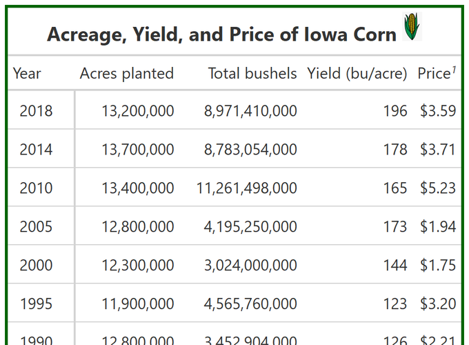
Acreage, Yield, and Price of Iowa Corn  |
||||
|---|---|---|---|---|
| Year | Acres planted | Total production | Yield (bu/acre) | Price1 |
| 2018 | 13,200,000 | $8,971,410,000.00 | 196 | $3.59 |
| 2014 | 13,700,000 | $8,783,054,000.00 | 178 | $3.71 |
| 2010 | 13,400,000 | $11,261,498,000.00 | 165 | $5.23 |
| 2005 | 12,800,000 | $4,195,250,000.00 | 173 | $1.94 |
| 2000 | 12,300,000 | $3,024,000,000.00 | 144 | $1.75 |
| 1995 | 11,900,000 | $4,565,760,000.00 | 123 | $3.20 |
| 1990 | 12,800,000 | $3,452,904,000.00 | 126 | $2.21 |
| Average | 12,871,428.57 | 6,321,982,285.71 | 157.86 | 3.09 |
| Source: USDA NASS | ||||
|
1
per bushel (equivalent to 64 pints)
|
||||
I added a darkgreen border to the whole table
I added a grand summary line at the bottom that takes the average of all columns. I couldn’t figure out how to get some of the columns with dollar signs and some without…?
I added a tiny corn image to the title! Which looked great when I saved the table as png (as you can see from image in this post), but then gets all messed up when rendered via blogdown.
Btw, tables are pretty easy to save:
# gtsave(last_tab, filename = "corn_table.png")
Again, let’s just take a quick moment to look at these numbers. Corn acreage has increased since 1990, peaking in 2014. Prices per bushel and total production ($) are highest in 2010 (thanks renewable fuel standard!), so it makes sense we’d see a delayed boom in production acres in 2014. Yield continues to steadily increase.